To calculate traveling wave accelerators (cavities), GPT[1] provides three built-in elements (trwcell, trwlinac, and trwlinbm). In these elements, the electromagnetic field of a traveling wave accelerator is handled as follows[2];
\begin{align} E_z&=E_0\sin(\omega t+\phi-k_zz)I_0(k_rr) \nonumber \\ E_r&=E_0\cos(\omega t+\phi-k_zz)I_1(k_rr) \\ B_\phi&= E_r/c \nonumber \end{align} where (\(E_z, E_r, B_\phi\)) are electric-magnetic fields.
Calculating a standing-wave cavity in GPT is easy. First, use the command sf7 and fish2gdf to create a gdf file describing the electromagnetic field. Then, the GPT read the field data from the SUPERFISH calculation. In contrast, the case of traveling wave accelerators is much more challenging to handle because SUPERFISH cannot calculate the traveling wave electromagnetic field, and the GPT cannot directly capture the traveling wave electromagnetic field. However, with some ingenuity, it is possible to handle traveling waves. Here, I would like to introduce a technique that I used. This technique is especially suitable for simulations of bunching low-energy (tens to hundreds [keV]) beams from electron guns with a traveling wave buncher. For beam tracking in a traveling wave accelerator at GPT, the structure design is shown in Figure 1. Half of the input and output couplers at both ends are standing waves (SW), and the rest are traveling waves (TW). In this way, the electromagnetic field in the area excluding the cavity of the coupler is almost the same as that in the actual accelerating tube. The electric field in the coupler will also be nearly the same as the actual field. There is a slight problem with the magnetic field, as I will explain later. When calculating a buncher tube, the electric field is more critical than the magnetic field, so the accuracy of the magnetic field is sacrificed.

Figure1: In the case of traveling wave accelerators, SW denotes the standing wave region, and TW means the traveling wave region.

Traveling Wave Region

As is well known, an expression of traveling waves is superimposing two electromagnetic fields with different boundary conditions. For example, a concrete accelerator tube is shown in Figure 2, with a 1.5 cell (1.5 periods) region and various boundary conditions at both ends. The boundary conditions at both ends are different: one is an electric short-circuit surface at both ends, and the other is a magnetic short-circuit surface. As a result, the electromagnetic field (eigenfunction) is different, but the frequency (eigenvalue) is the same. If the stored energies are the same (normalized) and superimposed with a phase change of \(\pi\)/2 [rad], we can form a traveling wave.

Figure2: Boundary conditions at both ends are short(SS)	Figure3: Boundary conditions at both ends are open(OO)

The electric and magnetic fields of a traveling wave are
\begin{align} E_{TW}(r,t)&=\left[E_{SS}(r,\omega)+iE_{OO}(r,\omega)\right]e^{i\omega t}\\ H_{TW}(r,t)&=\left[H_{OO}(r,\omega)-iH_{SS}(r,\omega)\right]e^{i\omega t} \end{align}
\(E_{TW}\) and \(H_{TW}\) represent the electromagnetic field of a traveling wave, \(E_{SS}\) and \(H_{SS}\) are the electromagnetic fields calculated by SUPERFISH when the boundary conditions at both ends are short (Figure 2), and \(E_{OO}\) and \(H_{OO}\) are the electromagnetic fields calculated by SUPERFISH when the boundary conditions at both ends are open (Figure 3). This Equation can calculate the electromagnetic field of a traveling wave from the standing wave that SUPERFISH can calculate.
Next, we consider the energy flow of the electromagnetic field. The power of the electromagnetic field to the left of the traveling wave region in the leftmost cell of the accelerating tube (input coupler side) is the input power of the accelerating tube. The energy of the electromagnetic field in the accelerating tube moves from the input coupler to the output coupler in the traveling wave region. Due to the finite Q of the cavity, the energy of the electromagnetic field decays as it moves. We calculate the dissipation per unit length by the group velocity \((v_g)\) and the Q value \((Q_0)\). If the direction of the travel in the accelerator tube is \(z\), the change in RF power \((P)\) is \begin{align} \frac{dP}{dz}=-\cfrac{\omega P}{v_gQ_0} \end{align} Therefore, for every one cell movement of the accelerator tube, the RF power decays at a rate of \(\exp(-\omega D/v_gQ)\), where \(D\) is the length of the one cell. The relationship between the stored energy \((U)\) and the group velocity is as follows \begin{align} \cfrac{v_gU}{D}=P \end{align} In the accelerating tube model shown in Figure 1, the stored energy in the region is taken into account for this attenuation when moving to the next traveling wave region (TW).

Standng Wave Region

Half of the coupler cell should be standing wave. In a real accelerating tube, both ends are standing waves. There is a change in the middle of the coupler cavity from a standing wave to a traveling wave and vice versa. Of course, this is different from a real accelerating tube. At these boundaries, we adjust the electromagnetic field in the standing wave region to continue the on-axis electric field. Then, the electric field can be almost constant over the boundary region. On the other hand, the magnetic field is a discontinuity (discrete) that is unavoidable as long as we use the model of Figure1.
The magnetic field in the TM mode affects the beam dynamics only when the particle velocity \((v)\) is smaller than the high speed. This effect is powerful in the vicinity of the input cavity of the buncher acceleration tube of an electron linac. However, the beam radius here is small in a real accelerator tube, so the effect is negligible. Nevertheless, compared to the magnetic field, the electric field has a much more substantial impact on the beam dynamics. Therefore, as shown earlier, at the boundary between traveling and standing waves, making the electric field continuous is better than making the magnetic field constant for a good approximation.

Programing

Here I am programming in Perl, referring to the page of my mentor, Mr. Yamamoto. For efficient calculation, it is necessary to calculate the traveling wave accelerating tube's electromagnetic field and automatically create the input file of the GPT. For this purpose, the author created two programs written in Perl: mk_TW_gdf_04B.pl, which makes a "*.gdf" input file for the electromagnetic field of GPT, and mk_GPTin_file.pl, which creates a part of the corresponding GPT input file "*.in". mk_TW_gdf_04B.pl starts SUPERFISH according to the input file and calculates the electromagnetic field in the accelerating tube. It automatically adjusts the cavity diameters and sets the frequency to 2856[MHz]. In the traveling wave region, calculate 1.5 cells as shown in Fig. 2 and Fig. 3, and convert the required 1-cell electromagnetic field into a GPT file (*.gdf) for storage. In the same way, calculate the standing wave region and store the electromagnetic field in a file. The parameters of the acceleration cell, such as the group velocity, stored energy, and Q-value, are stored in files (*.tw, *.sw). mk_GPTin_file.pl follows the input file and the output file (*.tw, *.sw) of mk_TW_gdf_04B.pl to create a part of the GPT input file (*.in), the line describing the traveling wave accelerator. Two text files (*.para, *.forGPT) will come out by executing this program. The former (*.para) contains the parameters of the accelerator. The latter (*.forGPT) is the traveling wave accelerator part of the GPT input file (*.in). Finally, we copy and paste the file into the GPT input file. As explained above, to create the input data for the traveling wave accelerator, you need to run the two programs mk_TW_gdf_04B.pl and mk_GPTin_file.pl in sequence.

How to use

Download here to get my scripts. In the TW_4B folder, you might have;

• A perl program to create GPT gdf files (mk_TW_gdf_04B.pl).
• A perl program to create GPT input files (*.in) (mk_GPTin_file.pl).
• A batch file (mk_file_TW.bat) that creates all the necessary files for GPT at once.
• An example of an input file for a traveling wave accelerator (TW_structure.dat).

In the GPT_dir folder you might have;

• A GPT input file (TW_Buncher.in).
• A batch file (run.bat)
• A perl program for phase plotting (mk_phase_plot.pl).
• A perl program for particle distribution (gdf2a_CutData.pl).
• A gunplot program for the energy distribution (E_hist.gp).
• GDT files for the GPT results.

For expecting the batch file, enter the TW_4B folder and command below;

>mk_file_TW.bat

The scripts generate the "*.gdf" files in the folder and TW_structure.forGPT file is important for the tracking simulation by GPT. For the batch file, we need input file as below;

Example of input file(TW_structure.dat)

$directory
../TW_4B/
$end
#------------------------------------------------------
$input_RF
4.0        #input RF power [MW]
$end
#------------------------------------------------------
$sw
#pipeL	2a
30.000	20.00
30.000	20.00
$end
#------------------------------------------------------
$cell
#beta	2a	2b	t	Num
0.700	22.000	83.158	5.000	1
0.800	21.900	83.515	5.000	1
0.900	21.800	83.493	5.000	1
1.000	20.000	83.470	5.000	27

The number sign "#" in the input file indicates a comment. If this symbol is present, the program ignores the rest of the line. The input file consists of four sections. The input file requires these sections below. Please refer to the input file above to understand the contents of the input data.

• Directory section
  • From $directory to $end is the directory section.
  • This section shows the directory of the gdf file describing the electromagnetic field, viewed from the GPT input file (*.in). The directory specification here only affects the directory of the gdf file described in the output file (*.para, *.forGPT) of mk_GPTin_file.pl.
  • ../TW_4B/ is specified in the input file example above. This means that the gdf file is stored in the subdirectory of TW_4B. If the GPT input file and the gdf file are in the same directory, specify ./ if the GPT input file and the gdf file are in the same directory.
• Input RF power section
  • The input RF power section is from $input_RF to $end.
  • Specify the input power [MW] of the traveling wave accelerator. The RF power specification affects the multiplication factor of the output file (*.para, *.forGPT). That means for the "ffac" factor of the GPT element "map25D_TM".
• Standing wave section
  • The standing wave section is from $sw to $end.
  • It describes the shape of the standing wave region of the input coupler and the output coupler in two lines. The first line is the input coupler and the second line is the output coupler.
  • The lines are tab-delimited and describe the length of the pipe section, followed by the diameter of the pipe section (Figure 4).
  • The corner \(R\) of the connection between the pipe and the cavity will be the same as the corner of the adjacent disk.
  • The diameter of the cavity will be the same as the diameter of the adjacent cavity.
  • The length of the cavity section is half of the adjacent cavity (one cell of the adjacent traveling wave).
• Traveling wave section
  • From$cell to $end is the standing wave section.
  • Each line is a cell of the traveling wave cavity.
  • Num means the number of cavities with the same parameters (beta, 2a, 2b, and t).
  • The lines are tab-delimited and are ordered by\(\beta=v_p/c\) and describe the disk hole diameter (\(2a\)[mm]), cavity diameter (\(2b\)[mm]) and disk thickness (\(t\)[mm]) (Figure 6).
  • The tip \(R\) of the disk is half of the disk thickness.
  • The cavity diameter (\(2b\)) is adjusted to be \(2\pi/3\) mode at the frequency of 2856[MHz]. In the program "mk_TW_gdf_04B.pl", the frequency is approximately 2856[MHz] by the order of \(10^{-6}\). The cavity diameter (\(2b\)) is just a starting point for the calculation.

Figure4: Structure diameters

GPT simulation

1. Create a directory for GPT calculations. Let's say the name of this directory is "GPT_dir".
2. Go to the parent directory of this GPT calculation directory and create a subdirectory "TW_4B" there. This is because the directory of the gdf file is "../TW_4B/" in the input file.
3. Move all the gdf files created in the previous section to this directory "TW_4B". (In my script, the gdf files are created in the "TW_4B")
4. Create a GPT input file ( *.in ) in the directory "GPT_dir", excluding the traveling wave accelerator part.
5. Open the file ( *.forGPT ) created by mk_GPTin_file.pl, in this case "TW_structure.forGPT", and copy it to the GPT input file.
6. Write the other necessary information in the GPT input file.
   • Write the variable mm for the length unit.
   • Define the angular frequency of the acceleration tube in the variable omega.
   • Define the center coordinate of the input coupler of the acceleration tube in the variableStrZ. The unit is [mm].
   • Define the initial phase of the acceleration tube in the variable StrP. The unit is [deg].
7. Then save the file with an appropriate name, in this case "TW_Buncher.in".

Now, create a batch file (e.g. run.bat) to run the GPT. In my batch file in "GPT_dir", the commands show below;

>gpt -o TW_Buncher.gdf TW_Buncher.in


>gdf2a -w 15 TW_Buncher.gdf x y z Bx By Bz G | perl gdf2a_CutData.pl position 1.1594 1.1599 > acc_part.dat


>perl mk_phase_plot.pl

This first command is for GPT simulation. The second command is for the out put of particle distributions between 1.1594 to 1.1599[m]. The third command is for the phase distribution shown in Figure5. If you have Gnuplot, you can command with the E_hist.gp file to get the figure of theenergy distribution (See Fig.6).

>gnuplot E_hist.gp

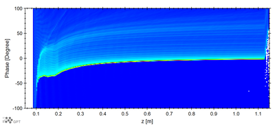
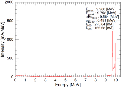
Figure5: Phase plots for the traveling wave accelerator. Figure6: Beam energy distribution at 1.1595[m].

References